 |
Frequently Asked Questions and User Guide
|
|
Frequently Asked Questions and User Guide
|
Due to some observed irregularities when it comes to the differences between area definitions in RAVE and the ones written to the ODIM H5 files we investigated these irregularities and also decided to write a document about the navigation within RAVE and how it compares to the ODIM H5 area definitions.
During the investigation the cause of the irregularity was found and due to that some changes has to be made related to the current RAVE area definition handling. Currently, the areas created by RAVE defines the outer boundaries without any adjustments of corners. However, when writing to ODIM H5 it is assumed that the boundaries have been adjusted.
The actual navigation is on the other hand working as expected with quite good accuracy.
A simple approach to solve the found inconsistency is to remove the adjustment of corner coordinates when reading and writing to the ODIM H5 format. This might cause some problems for users of the current ODIM H5 files since the UL/UR/LL and LR coordinates will be altered.
ODIM H5 specifies 4 different longitude/latitude pairs.
These coordinates defines the outer boundaries of the area covered. Besides these coordinate pairs, the area definition is also made up by xsize, ysize, xscale, yscale and a PROJ.4 projection definition. This is best illustrated with a picture.
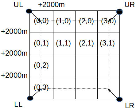
We define an area that we want to cover with 4 longitude/latitude pairs that defines the corners. These corners are Upper Left, Upper Right, Lower Left and Lower Right. However, these pairs will not be useful without a projection and this is defined as a PROJ.4 string. Since it is possible to translate from lon/lat to a metric scale when using the PROJ.4 library we only need to determine what xsize and ysize to get the xscale and yscale which in our example is 2000 meter. Obviously, this is not an ideal approach since it will give scales with a lot of decimals. To overcome this, it’s easier to just specify the Lower Left pair and then the scale and resolution and from that determine the other lon/lat pairs.
As you can see in the above picture the area has been divided into a 4x4 area with a 2000 meter resolution. Each point in the area is defined by a (X,Y) coordinate that is placed in the center of each sub area. Hence, the UL/UR/.. defines the actual outer boundaries of the area.
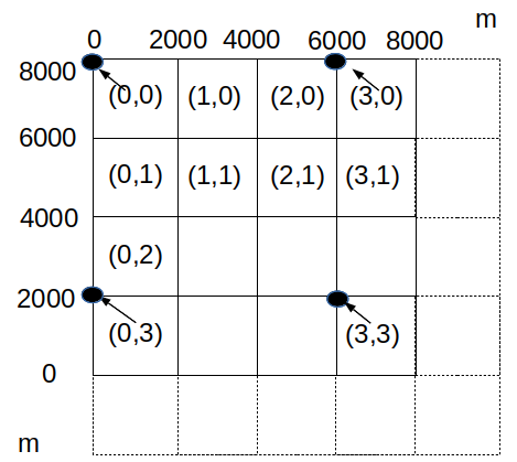
RAVE defines the area somewhat different when it comes to the area extent definition. Firstly, the areas extent is defined in meters according to the actual projection which means that the coorners are defined in a metric scale. Also, the only corners defined are lower left and upper right since the other corners can be derived from these two corners. The rest of the information is the same as defined in the ODIM H5 area definition. Namely, xsize, xscale, ysize, yscale and the PROJ.4 projection string. To simplify calculations and speed things up we have decided to move/transform the calculation points from center of the sub areat to the Upper Left corner. By doing this it is easy and fast to navigate and determine the actual longitude and latitude coordinates by using the following formula:
Since the formula is actually working on the upper left corner of each sub area it is tempting to change the formula somewhat and add half x & yscale.
However, we have not been able to see any improvments to the result. The reason for this is probably since most of the code is based on a nearest approach when transforming a polar scan/volume into the cartesian product and that the bins in the polar data is quite big. Any further investigation of the benefits of using half scale modification is left to the reader.
The easiest way to illustrate how the actual navigation is performed is with a picture. In the picture we can see that we are navigating in the matrix by using the upper left corner according to the formula specified earlier. This means that the upper left sub area coordinate will be (0, 8000) and the lower right corner will have (6000, 2000) as coordinate.
This doesn't mean that the area extent is any smaller. Just because the max coordinate in the area we cover is (6000, 2000) it doesn't mean that the area covered has changed. It is still from (0,0) to (8000, 8000). The reason for this is that we just have changed how we index the sub areas.
RAVE provides a tool called area_registry, that in turn uses the python script rave_area.py. This script takes one or more polar files, a PROJ.4 projection string, xscale and yscale and creates an area definition that covers these files. The approach is straight forward. The algorithm loops over all azimuths for each radar. Then it calculates the max and min x/y- position in the provided projection. After that it calculates the x and ysize from the provided scales and rounds upward so that the radar(s) are covered fully.
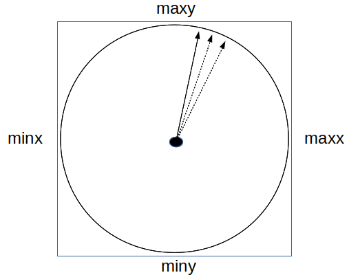
When minx,maxx,miny and maxy has been calculated. The xsize and ysize is determined by
Since the x & ysizes must be integer values and that dx & dy might be decimal number, the minx/maxx,miny and maxy might have to be adjusted outwards. Ie. minx/miny might become smaller and maxx/maxy might become bigger to ensure that the radar is fully covered by the area.
When this process has been performed the area definition that is created will be defined as follows.
To exemplify what the outcome from the auto generation of an area is, a quality controlled polar volume from Ängelholm, 20120131 has been used with scale 100.0 meters and the mercator projection identified as gmaps by using the function
| Attribute | Value |
| xsize | 8689 |
| ysize | 8700 |
| xscale | 100.0 |
| yscale | 100.0 |
| extent | 996171.309146, 7209261.288608, 1865071.309146, 8079261.288608 |
| pcsid | gmaps |
According to how MakeSingleAreaFromSCAN is written, the above extent is assumed to be the outer extent.
In order for rave to be able to use this area definition we will have to add it to the area registry. We can either do it manually by adding it to one of the area definition files in rave or use the tool area_registry.
The tool area_registry is a command line program that is invoked with a number of arguments. In our case we use it like this
The following printout will be displayed
testarea -      test area
        projection identifier = gmaps
        extent = 996171.309146, 7209261.288608, 1865071.309146, 8079261.288608
        xsize = 8689, ysize = 8700
        xscale = 100.000000, yscale = 100.000000
        South-west corner lon/lat: 8.948759, 54.205969
        North-west corner lon/lat: 8.948759, 58.529406
        North-east corner lon/lat: 16.755119, 58.529406
        South-east corner lon/lat: 16.755119, 54.205969
and the following entry will have been written to raves area_registry.xml file
  <area id="testarea">
    <description>
      test area
    </description>
    <areadef>
      <arg id="pcs">
        gmaps
      </arg>
      <arg id="xsize">
        8689
      </arg>
      <arg id="ysize">
        8700
      </arg>
      <arg id="xscale">
        100.000000
      </arg>
      <arg id="yscale">
        100.000000
      </arg>
      <arg id="extent">
        996171.309146, 7209261.288608, 1865071.309146, 8079261.288608
      </arg>
    </areadef>
  </area>
Both ODIM H5 and the Google map presentation uses outer boundaries as lon/lat coordinates for describing the area covered and earlier in this document it has been explained why it makes more sense to specify the generated extent with the outer boundaries as well. It is also worth to mention that if the test_areas extents corners are translated from the mercator projection into lon/lat they will become the same as used by the coordinates used in products.js that is generated in the GoogleMapsPlugin project.
| Product | Lower Left (Lon, Lat) | Upper Right (Lon, Lat) |
| area_registry | 8.948759, 54.205969 | 16.755119, 58.529406 |
| ODIM H5 | 8.94876, 54.206 | 16.7551, 58.5294 |
| Gmap products.js | 8.948759, 54.205969 | 16.754221, 58.528937 |
The difference is not big, but it’s due to the fact that when storing the ODIM H5 file, the upper left, upper right and lower right coordinate points are adjusted in northern/eastern direction to handle the assumption that the extent is covering from lower left corner to the lower left corner of the upper right sub area. Anyhow since both the ODIM H5 and Google Maps / Open streetmap assumes that the areas are limited by the outer boundaries one of the above two products must be erroneous. From earlier observations, it is clear that the ODIM H5 file should not be saved with any adjustments of the extent.
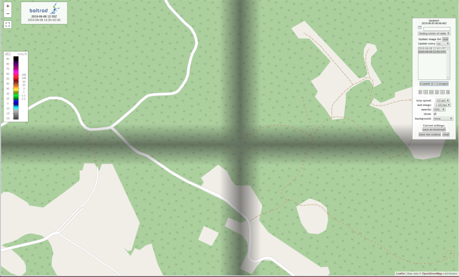
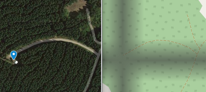
To validate how accurate RAVE is when it comes to navigation, a known reference point is needed as well as a validated map. Besides this, it is necessary to perform the navigation in a high enough resolution and this is quite time consuming since the areas will become quite big. The approach that has been used in this document is to use Ängelholm radar and create an automatic area definition. Add this definition to the area registry and also update the gmaps plugin with the generated coordinates for viewing in open street map. The resolution is 100x100 meter and the projection string “+proj=merc +lat_ts=0 +lon_0=0 +k=1.0 +R=6378137.0 +nadgrids=@null +no_defs”.
Then, a cross has been drawn into the image that has it’s center on the radars location. In the first picture you can see that the cross is shaded and that the darker shade is centered south of the end of a road. In the second picture you will see a side-by-side presentation of the created image compared with a map containing the location of the radar and you can see that the rave transformation seems to be doing a fairly good job.
 1.9.1 for