 |
Frequently Asked Questions and User Guide
|
|
Frequently Asked Questions and User Guide
|
Your node should now be receiving data from your own radar(s), and exchanging data safely and smoothly with other nodes. This is where you can learn more about how these data can now be processed. We will go the through the procedure of setting up data processing by using an example based on polar scans that arrive to a node individually, they are compiled into volumes, optionally quality-controlled, and then a Pseudo-CAPPI is generated. The resulting product file will be used to create a graphics image for web-based display. We finish by outlining how the BALTRAD toolbox can be used on the command line, with scripts, and how you can contribute to it.
Before we get into the details, we should probably touch on some of the principles that are applied when it comes to data processing in our system. In principle, data processing is an optional part of the overall node concept that have implemented. Take a look at the item in the FAQ addressing What are the system components and how to they interact?. You don't have to install your node with the packages containing data processing functionality. In that case, you won't have access to a lot of useful stuff, including some routines e.g. for Generating new keys and one of the data injectors that you can use for Getting your own data into your node.
The concept that we've applied to achieve this separation between the core system and data processing is that data processing takes place in a separate system that communicates with the core system over the wire. This means that the data processing can take place on another machine and still work together with your node. The only requirement in this case is that a common disk volume is shared. This can be done using a SAN or perhaps an NFS volume if it doesn't suffer from poor bandwidth. Revisit Requirements for more on this.
We should also clarify some of the terms used here. We have two Product Generation Frameworks (PGF) in BALTRAD, one written in Java and the other written in Python. The former is currently unused, as there has been no demand for it, but it is available anyway. This documentation will therefore focus on how to manage and use the Python PGF. This is the RAVE package, and RAVE combined with the other packages that work together with it are collectively referred to as the BALTRAD Toolbox.
A note on single-site vs. composite products. In the BALTRAD toolbox, there is currently no difference. All Cartesian products are composites, even if they contain data from just one radar. In all cases, polar data are nagivated directly to the output area with no intermediate steps or projections. We'll see how this works in practice later.
We distinguish between what kind of job we want a PGF to run, and how we want the PGF to run it. In this sense, we will define product generation tasks separately from different ways of performing quality control. This may seem a little confusing now, but we hope everything will become clear once you've read this chapter.
Another little conceptutal detail before we move on.
This is where the concept of Adapters and Routes is most clearly applied. In order to communicate with a PGF, the node uses an XML-RPC adapter. The node takes care of all scheduling and triggering of processes. When the criteria are fulfilled for triggering a job, an XML-RPC message is sent to the PGF, telling it which algoritm to run, with which arguments, and with which input data. When the PGF has run the job, the resulting ODIM_H5 file is injected back into the node. Alternatively, some types of jobs, e.g. generating PNG images for Google Maps, don't inject data to the node because there's no need to.
You can process any data unless you have have some. By now, you should have followed the instructions on how to Add a radar or several.
Similarly, you will need to select input data based on the ODIM source node identifier, so you should Add ODIM source definitions to your node if you haven't already.
The first step in the data processing chain is to define an adapter so that the node knows where to find your PGF. In the web-based user interface, go to "Processing" --> "Adaptors" and press "Create". Assuming a default configuration, define a RAVE adapter like this:
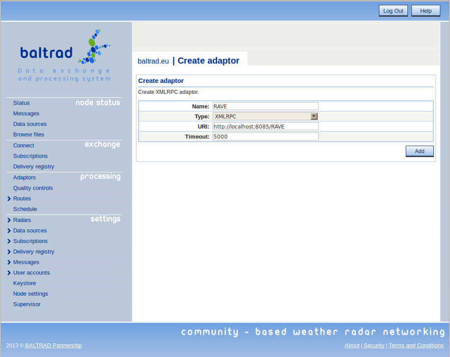
You can define several such adapters, even distributed among different machines, and you can then send different types of jobs to each. If you try this, ensure that these machines all share a common file system with your node as was mentioned in Background.
This may seem a little odd, but the modular nature of our system implies that it cannot be taken for granted that all ways of processing data have been installed when you built your node. Different packages exist for processing data in different ways. Two such packages are bRopo, a package that identifies and removes non-precipitation echoes ("anomalies") in polar data, and beamb, a packages that determines beam blockage caused by topography and corrects for it. In the case of bRopo, the original code base is large enough to justify managing it as a separate package. In the case of beamb, there are large digital elevation models that are included and that the algorithms rely on, so this is another justification for separate packaging.
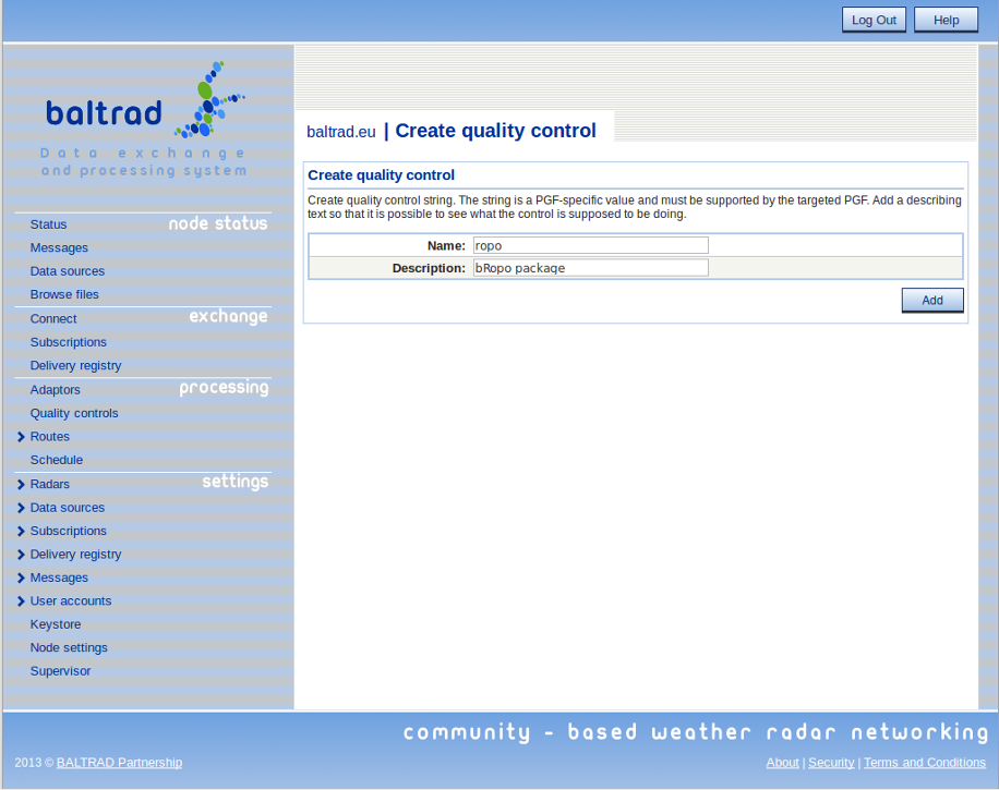
Define a quality control by going to "Processing" --> "Quality controls" and pressing the "Create" button, e.g. for the bRopo package:
This is a little tricker than it first seems, because the PGF must recognize the "Name" that you have entered. There are several quality controls available and might differ depending on what product generator that is used and what components that has been installed.
At the time of this documents writing, the following quality controls are available:
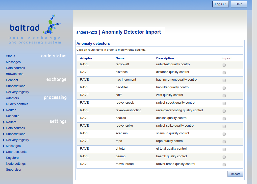
However, from release 2.2 you are also able to import the available quality controls from the registered product generators if the PGF has implemented support for returning the available quality controls.
You can reach this by going to "Processing" --> "Quality controls" and press the "Import" button.
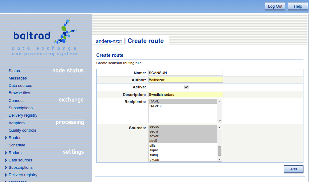
This is where we actually start doing something with data. The Route concept can also be referred to as a rule, where you define the criteria that need to be satisfied to start a data processing job. A volume route is not as trivial as it seems at face value, because it must be easy to configure but also contain enough intelligence to deal with scan strategies that change without notice, and scans that don't arrive for whatever reason.
Our volume route is adaptive which makes it pretty robust. The only details you need to provide that are related to the scan strategy itself are the lowest and highest elevation angles, and the repeat cycle. The route will then figure for itself out the other details. This means that it won't manage very well in cases where the scan strategy changes every cycle. In such cases, it is better to define separate routes for each type of scan strategy.
Here is an example of a volume route used with Swedish data.
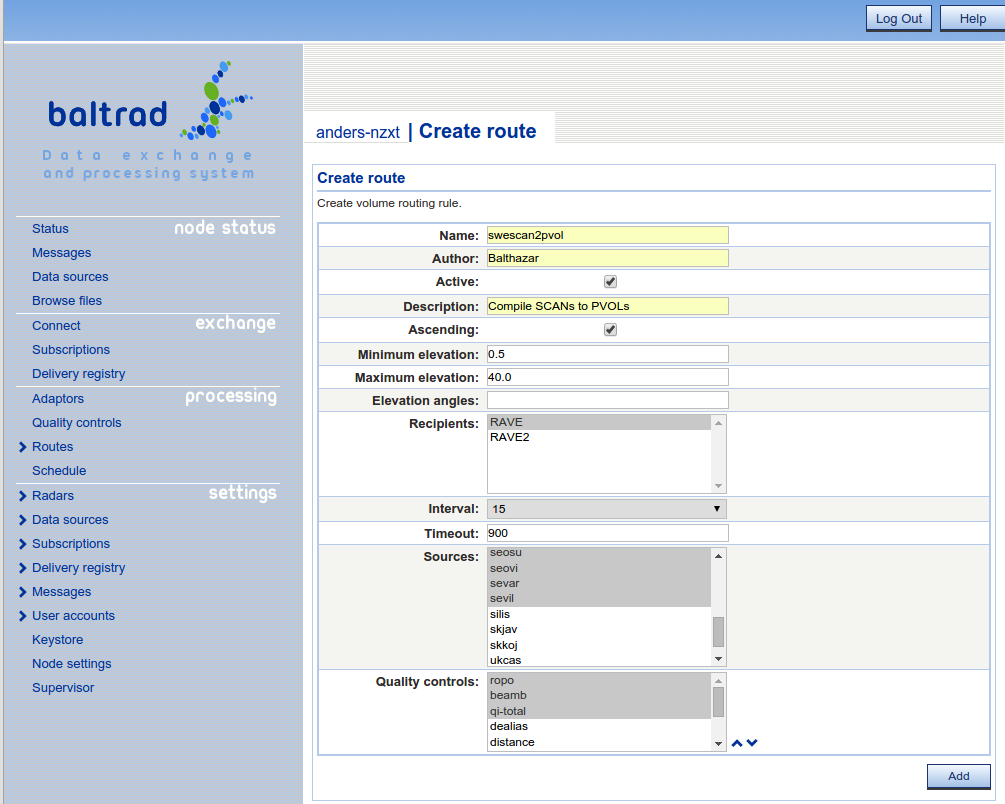
As soon as the bottom scan is received, the rule will activate and will monitor inbound scans from any of the selected sources. As soon as the top scan is received for a given source, the job will run. The timeout of 900 seconds (15 min) is very generous and can be reduced. If the top scan hasn't been received before the timeout is reached, then the volume will be created with those scans that have been received.
Quality control can be combined in the volume route, by selecting them when configuring the route. It is important to remember that the quality controls will be performed in the order they are selected in the selection list. Use the up and down arrows to arrange them properly.
Note that the routes never buffer data in memory, they only keep track of the whereabouts of the input data files through the metadata that was mined from them when the files arrived to the node.
When the route's criteria have been fulfilled, an XML-RPC message to the PGF will be triggered, and the PGF will compile the volume from the input scans, quality controlling them if this has been selected, and then inject the resulting volume into the node.
BALTRAD software uses the PROJ.4 projections library to navigate data. In the toolbox, there are tools available to help you do this. Normally, we would refer directly to the PGF's own documentation for the details, but this is a topic that is so fundamental to data processing that it's justified to cover it here.
This can be done on the command line using the projection_registry tool. The procedure is a rather transparant interface to PROJ.4, so you are referred to the PROJ.4 documentation regarding how it works.
The following example defines the projection used by Google Maps and adds this projection to the toolbox's projections registry:
$ projection_registry --add --identifier=gmaps \
--description="Google Maps" \
--definition="+proj=merc +lat_ts=0 +lon_0=0 +k=1.0 +R=6378137.0 +datum=WGS84 +nadgrids=@null +no_defs"
You can then verify that this definition has been added to the registry by running
$ projection_registry --list
and you should see the following entry:
gmaps - Google Maps
        +proj=merc +lat_ts=0 +lon_0=0 +k=1.0 +R=6378137.0 +datum=WGS84 +nadgrids=@null +no_defs
Now that you have this projection, you can define areas using it.
A projection is a two-dimensional representation of the Earth's shape. But we also need to know which part of the Earth we want to work with, and this is referred to as an area.
Defining an area and adding it to the toolbox's area registry is done using the area_registry command. If you already know your area definition and how it related to your projection definition, then just just use the command.
You can also use the tool to help you define an area that is based on the characteristics of your radar data, either a single radar or several to define a composite area, for example. In the following example, we use a polar volume of data from the Swedish radar located near Vara, inland from Gothenburg. First we determine a matching Cartesian area that uses the Google Maps projection we defined above.
But before we do that, we must know the real resolution we want on the Earth's surface. This is determined through knowledge of the latitude of true scale (lat_ts, in radians), as
projection_resolution(m) = ground_resolution(m) x 1 / cos(lat_ts)
Our radar is close to 60 degrees north, so let's use this latitude of true scale for the same of simplicity. If we want a real resolution on the ground of one kilometer, the projection's resolution will be two kilometers. Convenient. This is used when defining the Cartesian area:
$ area_registry --make --identifier=sevar_gmaps \
--description="Google Maps area for Vara" --proj_id=gmaps --files=sevar.h5 \
--xscale=2000.0 --yscale=2000.0
This should print out the following:
__PROVISIONAL__ -       Area using projection with identifier "gmaps"
        projection identifier = gmaps
        extent = 967050.466007, 7575120.949412, 1887050.466007, 8495120.949412
        xsize = 460, ysize = 460
        xscale = 2000.000000, yscale = 2000.000000
        South-west corner lon/lat: 8.687162, 56.083825
        North-west corner lon/lat: 8.687162, 60.434520
        North-east corner lon/lat: 16.969629, 60.434520
        South-east corner lon/lat: 16.969629, 56.083825
Run again with -a -i <identifier> -d <"description"> to add this area to the registry.
Re-running but using the –add argument and this output will register this area:
$ area_registry --add --identifier=sevar_gmaps \
--description="Google Maps area for Vara" --proj_id=gmaps  \
--xscale=2000.0 --yscale=2000.0 --xsize=460 --ysize=460 \
--extent='967050.466007, 7575120.949412, 1887050.466007, 8495120.949412'
Verify by running:
$ area_registry --list
and you should see the following entry:
sevar_gmaps -   Google Maps area for Vara
        projection identifier = gmaps
        extent = 967050.466007, 7575120.949412, 1887050.466007, 8495120.949412
        xsize = 460, ysize = 460
        xscale = 2000.000000, yscale = 2000.000000
        South-west corner lon/lat: 8.687162, 56.083825
        North-west corner lon/lat: 8.687162, 60.434520
        North-east corner lon/lat: 16.969629, 60.434520
        South-east corner lon/lat: 16.969629, 56.083825
The corner coordinates will come in handy later, so keep them in mind.
Note that if we had used area_registry with several files as input, then the resulting area definition would have been a composite area including all radars' coverage areas.
We now have all the information we need to generate a Cartesian product for our example. This is done through the web-based user interface, by going to "Processing" --> "Routes" --> "Create composite".
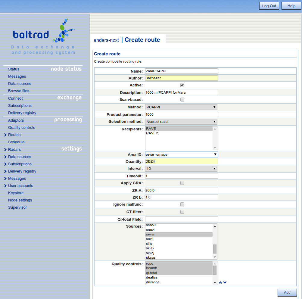
Note that the "Product parameter" is modelled after the same metadata attribute in ODIM.
When selecting areas you can get a list of areas from the available PGFs by double clicking in the text field provided that the PGFs are able to return available areas.
Prodpar is not used in the composite route as a selection filter. It only provides the PGF with a value to use during the product generation. That means that there is a limitation on the PPI method, only the lowest elevation will be used as a selection criteria if SCAN-based selection has been chosen.
The observant reader will probably recognize that the PVOL route above also was registered to execute ropo, beamb and qi-total as quality controls. RAVE is able to detect that a specific quality control already has been executed so if RAVE is the intended target, the quality control will not be rerun if the specified quality controls already has been executed.
You are able to perform additional stuff on the generated products, for example Gauge Radar Adjustment (GRA) which you can read more about in another section.
QI-total field is a somewhat different way of determining the composite. If specifying a class, then the radars used in the composite will be based on best quality. If using the default qi-total quality control, the name of the class to use is pl.imgw.quality.qi_total.
With this example, we have shown how single-site Cartesian products are generates as "Composites". This may seem a little counter-intuitive, but it works. Everything's a composite ...
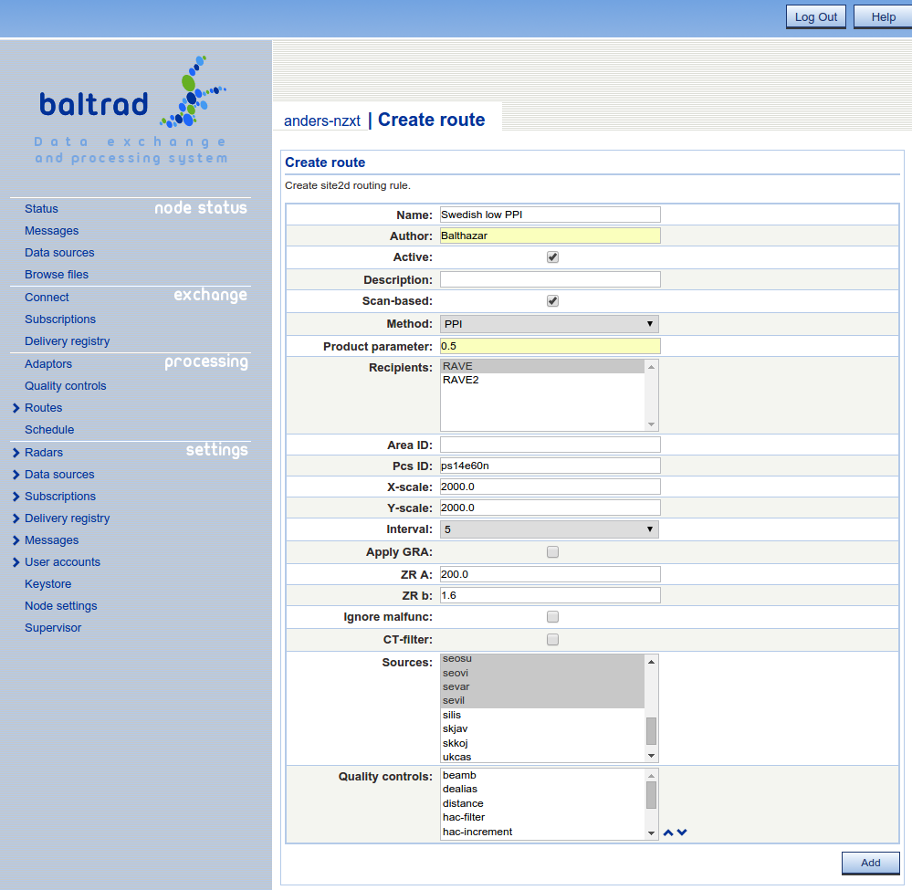
If you want to generate single site cartesian products you can use the Site 2D route instead. It almost works like the composite route with a couple of exceptions.
First, it triggers immediately when a source arrives matching the source-name and the prodpar. This means that when specifying PPI, prodpar and SCAN-based. The exact angle as specified in prodpar will be used.
Secondly, you can specify a Pcs ID and x-/y-scale instead of area and then a best-fit will be done.
We now have our node generating products in real time, so we might be interested in looking at them. BALTRAD doesn't contain its own visualizer. This is because different organizations have different visualization tools and strict policies governing them. So we decided we wanted a web-based display that would keep things simple. And it became easy to take a closer look at Google Maps.
If you built and installed your node with the –with-rave-gmap argument, then you already have the package installed. There are a few things you need to do manually before this service will work for you.
First thing to do is preparing a file containing geographic area definitions to use with the Google Maps plugin. To generate areas definition file, do the following:
%> cd $prefix/rave_gmap/web
%> source $prefix/etc/bltnode.rc
%> python ../Lib/GenerateProductInfo.py smhi-areas.xml
smhi-areas.xml might be a bit confusing, but it actually contains different product definitions. \endnoteAssuming that all went fine, a file called products.js will be created in $prefix/rave_gmap/web directory. It contains some area definitions we have used while developing the system. They can be replaced with your new one, or your new one can be added - refer to Configuring the plugin itself section to learn how to do that.
Next, make sure your web server knows about this plugin. We have integrated against an Apache server, so the instruction is valid for it. At the bottom of your server's httpd.conf file, add the following entry. This is assuming that you've checked with your system administrator what want to do won't conflict with anything they're already doing. We also assume that the Google Maps Plugin has been installed in the default location.
<VirtualHost *:80>
  DocumentRoot /opt/baltrad/rave_gmap/web
  ServerName balthazar.smhi.se
</VirtualHost>
After this, restart your Apache server:
root# service httpd restart
In case your system doesn't come with pre-installed apache server, or for some reason you need a custom setup, you might want to install it manually. Here are the steps necessary to install apache2 web server under Ubuntu operating system.
First, install the required packages:
sudo apt-get install apache2
sudo apt-get install php5
sudo apt-get install libapache2-mod-php5
Then point the server to the right DocumentRoot directory. In order to achieve this, edit the following configuration file:
/etc/apache2/sites-available/default
Set the DocumentRoot option so it points to your web data directory:
DocumentRoot /opt/baltrad/rave_gmap/web
Save the file and restart your web server:
sudo service apache2 restart
If you for example can not get the google map viewer to show the pictures you might have to configure so that index.php is found when browsing directories. There are a couple of locations where this setting can be placed. First, check in httd/conf.d/php.conf if there is an entry in that file reading 'DirectoryIndex index.php'. If not, you might have to modify the above described VirtualHost entry and add 'DirectoryIndex index.php' to the same. Save the file and restart your web server.
Define a route in the node for generating images for Google Maps. This is done by selecting "Routes" -> "Create Google Map" from the "Processing" section of the main menu. Remember to make sure that the "Area" and "Path" field values are correct:
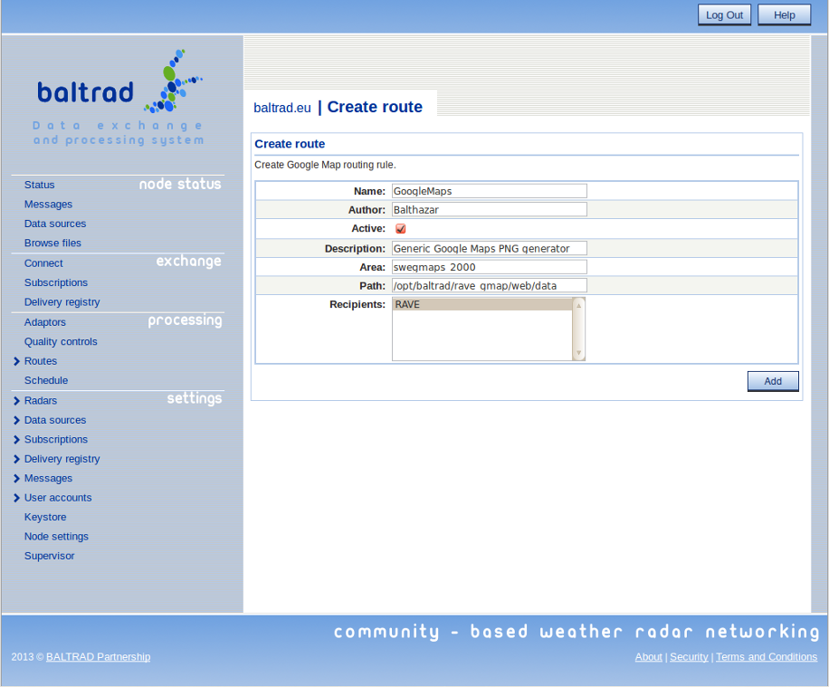
As soon as you have saved this route, the plugin will generate a PNG image for Google Maps each time an input file for it is generated.
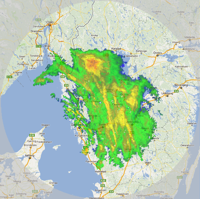
The final step is for you to configure the plugin itself, so that it contains a selectable product menu item that matches the product you're generating. We will use products.js file that you've generated in Configuring your web server section. As was mentioned above, the file contains some default area definitions. They can be replaced with your new one, or new one can be added. Continuing with our example from Vara, a corresponding entry for it makes use of the corner coordinates we determined earlier in Defining a Cartesian area and the radar's location:
//Product sevar_gmaps, Vara 1 km
radar_products['sevar_gmaps'] = new RadarProduct;
radar_products['sevar_gmaps'].description = 'Vara - Sweden';
radar_products['sevar_gmaps'].lon = 12.826;
radar_products['sevar_gmaps'].lat = 58.256;
radar_products['sevar_gmaps'].zoom = 5;
radar_products['sevar_gmaps'].nelon = 16.969629;
radar_products['sevar_gmaps'].nelat = 60.434520;
radar_products['sevar_gmaps'].swlon = 8.687162;
radar_products['sevar_gmaps'].swlat = 56.083825;
radar_option_list[1] = 'sevar_gmaps';
If you want to make this product the default that's displayed, make it first on the list, as radar_option_list[0]. Save the file and then use your browser to access Google Maps from your machine. Voilà!
Note that there are currently no routines for determining the maximum size of the disk space or age of the files used for storing PNG images. It's up to you to deal with this.
If you are interested in displaying images similarly using Web Map Services, check out the BALTRAD WMS package.
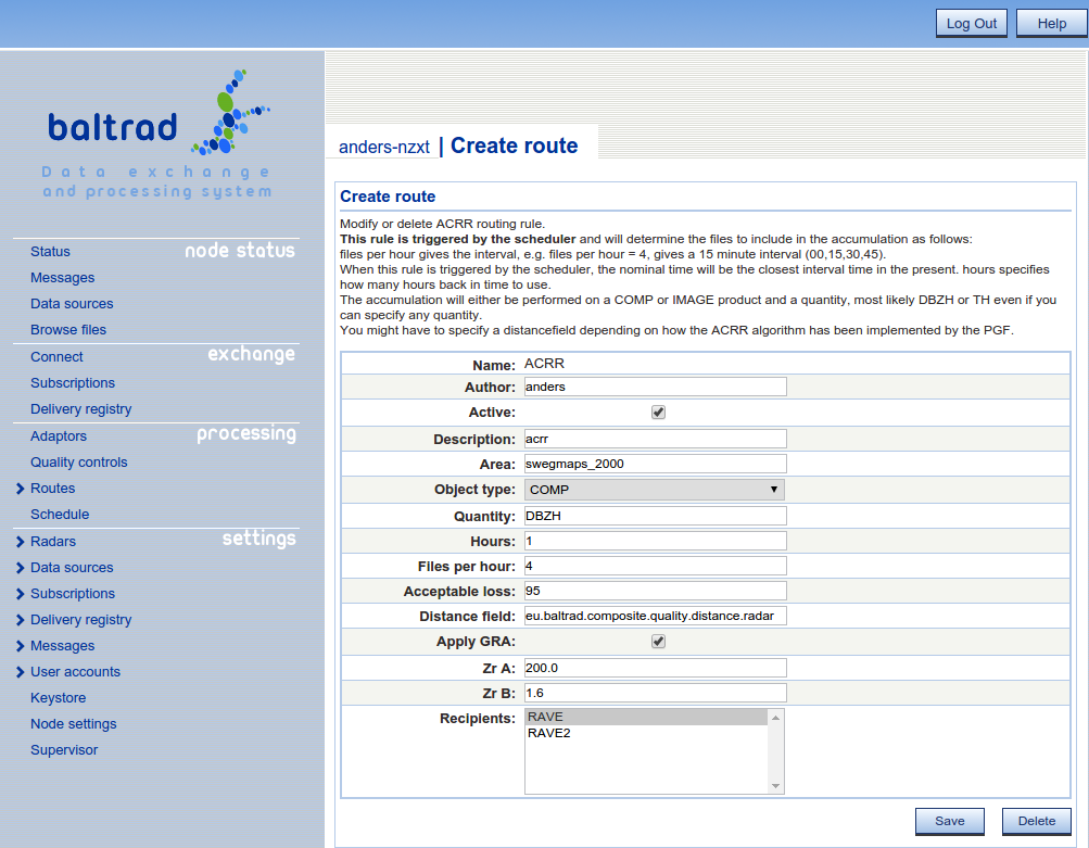
The accumulation of rain rate products is done somewhat different than the routes explained previously. Instead of files triggering the job, the job is triggered by a scheduler. So besides creating the route you will have to add a scheduled job.
There are a number of things that the user has to be aware of when creating the ACRR rule.
After you have setup the ACRR route. It is time to setup the schedule. The easiest way to do this is to use the provided scheduler in the user interface.
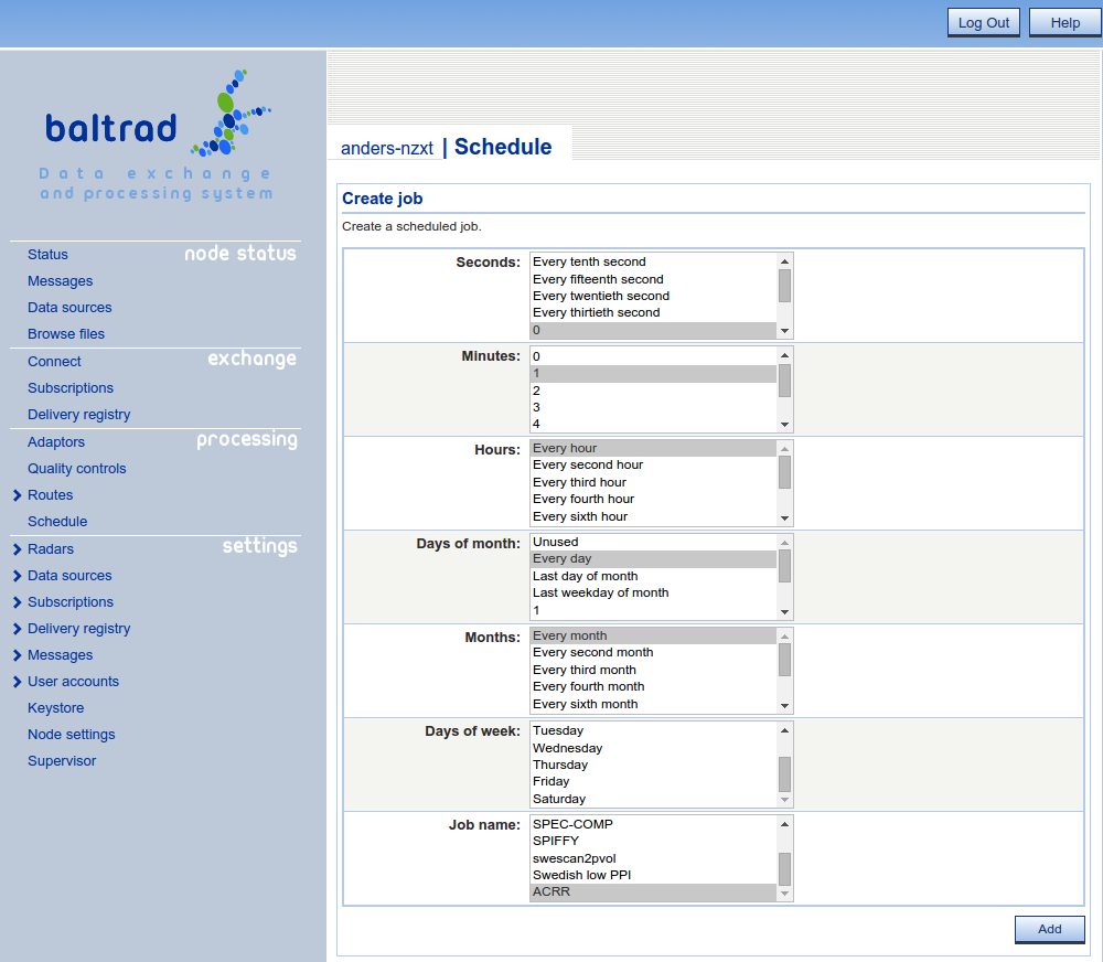
Note, that if you specify for example 1 hour, it might be a good idea to setup the scheduler to be run every hour but a couple of minutes after the nominal time. For example 00:02, 01:02 and so forth so that the composites are available.
If you for some reason want to use an external scheduler like crontab, you can create a small python script that invokes the ACRR route by using the injector functionality.
import BaltradFrame

if __name__ == "__main__":
  msg = """
<blttriggerjob>
  <id>999</id>
  <name>ACRR</name>
  <arguments></arguments>
</blttriggerjob>
"""
  BaltradFrame.send_message(msg, "http://localhost:8080/BaltradDex")
The ID is just for traceability so this can be whatever. The name is the name of the route. NOTE: Most of the routes does not support triggering.
The Gauge Radar Adjustment (GRA) is used for generating adjustment coefficients that can be applied in different algorithms like compositing and acrr.
In order to be meaningful, SYNOP-data has to be available. In the case of the rave PGF we have added support for handling observations in the FM12-format. If you have a different format, then you can write your own handler importing the observations into the database. The table containing the observations is named rave_observation and can be accessed by using the rave dom object rave_dom_db.rave_observation.
If you want to try to use the functionality provided by rave to import the synop data in FM12 format you will be using the fm12_importer script in the rave bin folder. But first, you need to get the fm12 messages somehow. One alternative is to subscribe them from GISC. The fm12_importer is using inotify for monitoring one folder so the fm12 messages should be placed in that folder.
Before you start the fm12_importer daemon you will also have to setup information about the stations that are delivered in the fm12 messages. This can be done by importing a flatfile containing all stations. You can find the flatfiles and other useful information here http://www.wmo.int/pages/prog/www/ois/volume-a/vola-home.htm.
Download the most recent file and import it with the following command
%> python bin/wmo_station --uri=postgresql://<dbuser>:<dbpwd>@<dbhost>/<dbname> --flatfile=<flatfile> import
When that has been done, it's just to start the fm12 importer daemon.
%> /opt/baltrad/rave/bin/fm12_importer --monitored=/gisc/fm12 --pidfile=/opt/baltrad/rave/etc/fm12_importer.pid
  --logfile=/opt/baltrad/rave/etc/fm12_importer.log --catchup --janitor daemon
As you can see, the command is quite self-explanatory. A couple of notes might be in order though.
\subscection rave_pgf_gra Creating the GRA route The GRA route is very similar to the ACRR route in both how it behaves and that it is triggered by a scheduler.
The distance field is very important and the composites has to have been generated with a distance-quality control. If you are using the distance anomaly detector that is provided by rave, the distance field should be named eu.baltrad.composite.quality.distance.radar.
First term UTC is used to define when the accumulation period should start. For example, if First term UTC is 6 and interval is 12, the periods will be 0600-1800, 1800-0600 and so on. Since the synops might arrive later than for example 0600, we have scheduled the coefficients to be run one hour later, i.e. at 0700 and 1900.
If you are using the Rave PGF you should be aware that the coefficients can be generated for any area but they will be the same for all GRA adjustments. Hence, just have one GRA route that uses a decently sized area.
NOTE: It is not relevant to specify a too small interval, a good interval is probably 12 hours. That also correlates with the 12-hour synop.
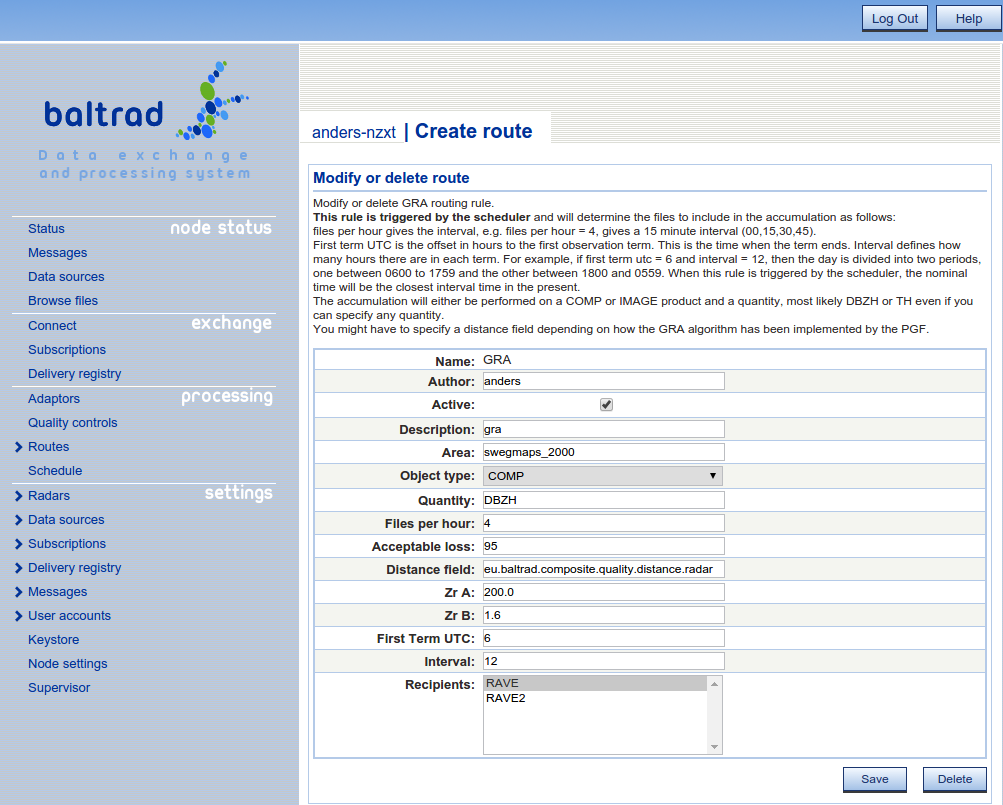
When you have setup and scheduled the GRA route to be executed the gra-coefficients will be generated. Since the number of radar-gauge observations will be quite small at any given time we are using a merge period of a number of terms. This can be defined in the variable MERGETERMS in rave/Lib/rave_defines.py. The current value assumes a 12-hour interval and 20 terms giving a 10 day period for calculating the gra coefficients.
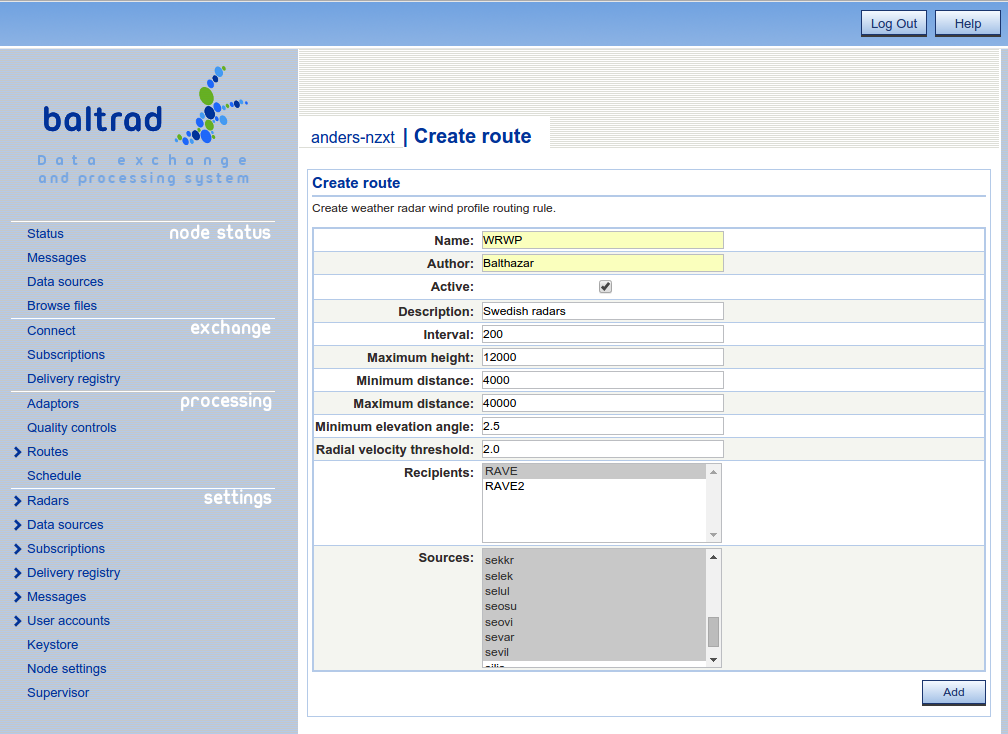
The route for generating wind profiles is quite simple. It is triggered on volumes for the specified sources. When a polar volume for that source arrives the PGF is notified and then a vertical profile is generated and injected back into the system.
The interval in this case is specifying how meters each section should be up to the maximum height. So in the case of max height = 12000 and interval = 200 the number of sections will be 60.
We have added a route for scanning polar volumes for sun hits. The result of this route beeing triggered is that a log file with hits will be created for each radar source.
You can find the resulting files in <install prefix>/rave/etc/scansun/.
In some cases, the routes we have predefined are not enough for whatever reason. They might not be flexible enough, not able to trigger on what you want or you might want to create a scheduled composite. In all these cases there is a solution but it will require some work from your side.
There is a route called Create script that is used for adding your custom rules written as groovy scripts. You can read more about how you can write a groovy script in the manuals describing the BEAST API.
As an example, we recently got a question if we are able to support composite generation that includes files within a specific time span ignoring the nominal time and sure we do, here you have an example that you can adjust according to your needs. Since this is a type of route that is not practical to trigger on incoming data it should be scheduled.
When you have modified it for your needs it's just to copy-paste it into the text area in a script route.
package eu.baltrad.scripts

import eu.baltrad.beast.rules.IScriptableRule;
import eu.baltrad.beast.message.IBltMessage
import eu.baltrad.beast.message.mo.BltGenerateMessage;
import eu.baltrad.beast.message.mo.BltTriggerJobMessage
import org.apache.log4j.Logger;
import org.apache.log4j.LogManager;

import eu.baltrad.bdb.db.FileEntry;
import eu.baltrad.bdb.db.FileQuery
import eu.baltrad.bdb.db.FileResult;
import eu.baltrad.bdb.expr.Expression;
import eu.baltrad.bdb.expr.ExpressionFactory
import eu.baltrad.bdb.oh5.Metadata;
import eu.baltrad.bdb.util.DateTime
import eu.baltrad.bdb.util.Date
import eu.baltrad.bdb.util.Time
import eu.baltrad.bdb.util.TimeDelta
import eu.baltrad.beast.ManagerContext
import eu.baltrad.beast.db.Catalog
import eu.baltrad.bdb.FileCatalog;
import eu.baltrad.bdb.db.Database;

class ScheduledComposite implements IScriptableRule {
        private static String AREA="swegmaps_2000";
        private static String[] SOURCES=["seang","searl","selul","sekkr"];
        private static String SELECTION = "NEAREST_RADAR"; // NEAREST_RADAR or HEIGHT_ABOVE_SEALEVEL
        private static String QC = "ropo,beamb";
        private static String METHOD = "ppi"; // ppi, cappi, pcappi, pmax or max
        private static String PRODPAR = "0.5";
        private static String QUANTITY = "DBZH";

        private static Logger logger = LogManager.getLogger(Ireland5MinuteComposite.class);

        ExpressionFactory xpr;
        List sources = new ArrayList();
        Expression dateTimeAttribute;
        Formatter formatter;

        Ireland5MinuteComposite() {
                xpr = new ExpressionFactory();
                formatter = new Formatter();
                dateTimeAttribute = xpr.combinedDateTime("what/date", "what/time");
                for (String src : SOURCES) {
                        sources.add(xpr.literal(src))
                }
        }

        @Override
        public IBltMessage handle(IBltMessage message) {
                if (message instanceof BltTriggerJobMessage) {
                        logger.info("Handling scheduled composite job");
                        return doHandle();
                }
                return null;
        }

        protected IBltMessage doHandle() {
                DateTime now = getNow();
                ArrayList<Expression> filters = new ArrayList<Expression>();
                filters.add(xpr.eq(xpr.attribute("what/object"), xpr.literal("PVOL")));
                filters.add(xpr.eq(xpr.attribute("what/quantity"), xpr.literal("DBZH")))
                filters.add(xpr.in(xpr.attribute("_bdb/source_name"), xpr.list(sources)))
                filters.add(xpr.ge(dateTimeAttribute, xpr.literal(getStartFromNow(now))))
                filters.add(xpr.le(dateTimeAttribute, xpr.literal(getEndFromNow(now))))

                FileQuery query = new FileQuery();
                query.setFilter(xpr.and(filters));

                ArrayList<String> files = new ArrayList<String>();
                FileResult set = null;
                try {
                        set = ManagerContext.getCatalog().getCatalog().getDatabase().execute(query);
                        while (set.next()) {
                                FileEntry fEntry = set.getFileEntry();
                                Metadata metadata = fEntry.getMetadata();
                                logger.info("Adding file: " + metadata.getWhatObject() + " " + metadata.getWhatDate() + " " + metadata.getWhatTime() + " " + metadata.getWhatSource());
                                files.add(fEntry.getUuid());
                        }
                } catch (RuntimeException t) {
                        t.printStackTrace();
                } finally {
                        if (set != null) {
                            set.close();
                        }
                }

                BltGenerateMessage result = new BltGenerateMessage();
                result.setAlgorithm("eu.baltrad.beast.GenerateComposite");
                result.setFiles(files as String[]);
                DateTime nominalTime = ManagerContext.getUtilities().createNominalTime(now, 5);
                Date date = nominalTime.getDate();
                Time time = nominalTime.getTime();
                result.setArguments([
                        "--area="+AREA,
                        "--date="+new Formatter().format("%d%02d%02d",date.year(), date.month(), date.day()).toString(),
                        "--time="+new Formatter().format("%02d%02d%02d",time.hour(), time.minute(), time.second()).toString(),
                        "--selection="+SELECTION,
                        "--anomaly-qc=" + QC,
                        "--method=" + METHOD,
                        "--prodpar=" + PRODPAR,
                        //"--applygra=true",
                        //"--zrA=200.0",
                        //"--zrb=1.6",
                        "--ignore-malfunc=true",
                        //"--ctfilter=True",
                        //"--qitotal_field=pl.imgw.quality.qi_total",
                        "--quantity=" + QUANTITY
                        ] as String[])

                for (String s : result.getArguments()) {
                        logger.info("Argument = " + s);
                }

                return result;
        }

        protected DateTime getNow() {
                return DateTime.utcNow();
    }

        protected DateTime getStartFromNow(DateTime dt) {
                return dt.add(new TimeDelta().addSeconds(-(7*60)));
        }

        protected DateTime getEndFromNow(DateTime dt) {
                return dt.add(new TimeDelta().addSeconds(-10));
        }
}
Some of the tools in the toolbox are available on the command line, which is useful for off-line work. To ensure that you have your environment set correctly before using them, make sure you have sourced the $prefix/etc/bltnode.rc file. Then, you can check out the bin directories of the various packages you have installed and see what's available. For example, you might be interested in determining whether a polar volume of data contains a sun signature.
$ scansun polar_volume.h5
An example from a Dutch radar should give e.g.
#Date    Time   Elevatn Azimuth ElevSun AzimSun dBmMHzSun dBmStdd RelevSun Source
20110111 075022    0.30  126.50   -0.78  126.84   -113.31  0.6722    -0.19 RAD:NL51,NOD:nldhl
This tool is prepared for monitoring sun "hits" assuming your input data are in ODIM_H5 version 2.1 with the required metadata.
Then, there are another tool called radarcomp. This is used for generating composites from scans and volumes. It allows the user to specify what quality controls that should be performed. If the composite should be performed with multiprocessing enabled and so on. For all options type
%> radarcomp --help
The bRopo package provides a tool for detection and removal of non-precipitation echoes ("anomalies"). A "lazy" use of it, where all input arguments and values are looked up from a file containing them is:
$ ropo -i input_volume.h5 -o output_volume.h5 --lookup=True
An example result is displayed in How do I use the BALTRAD toolbox interactively?. Run
$ ropo --help
to get a full listing of options.
Scripting is an effective development method. Not only does it allow rapid prototyping, it also reduces the bottlenecks in transforming a lab result to an operational implementation. There are also other bottlenecks that are addressed here, related to performance. By reading input data once, and then running all data processing on those data before writing the result once, we can speed things up remarkably. We do this with Python scripts, but they are just a thin layer on top of the underlying C which is the real engine.
The following example script does almost the same thing as the real-time routines we set up earlier. We use the same data as earlier too.
#!/usr/bin/env python
## Example of using a script to process data and chain algorithms in memory
import sys
import _raveio
import _transform
import ropo_realtime
import rave_composite
import rave_ql
def process(input_file, output_file):
# Read ODIM file and get its payload
io_container = _raveio.open(input_file)
polar_volume = io_container.object
# Detect and remove non-precipitation echoes. This generator is the "lazy"
# alternative, equivalent of using --lookup=True on the command line.
cleaned_volume = ropo_realtime.generate(polar_volume)
# Generate single-site 1 km DBZH Pseudo-CAPPI "composite"
composite = rave_composite.generate([cleaned_volume], area="sevar_gmaps",
quantity="DBZH",
product="PCAPPI",
prodpar=1000.0,
method="NEAREST_RADAR")
# Perform rudimentary (1 pixel) gap-filling on the composite
t = _transform.new()
gap_filled = t.fillGap(composite)
composite.setData(gap_filled.getData())
# Display a quick-look window of the result
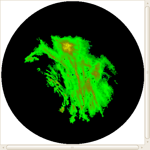
rave_ql.ql(composite.getData())
# Recycle the I/O container and write output ODIM_H5 file
io_container.object = composite
io_container.filename = output_file
io_container.save()
if __name__ == "__main__":
# No validation of arguments
process(sys.argv[1], sys.argv[2])
The quick-look window looks like this. It uses a different color palette than the Google Maps image above.
This also illustrates the value of using common routines to read and write data, because chaining algorithms from different contributors in memory like this is impossible otherwise.
We are part of a community that benefits through cooperation. We would love to see this community grow, and one way of doing this is to get involved and contribute a processing algorithm. In doing so, there's a golden rule that we want to note: separation of file I/O and the data processing. This means that the data processing functionality should not be mixed with the functionality used to read and write the data to/from disk. Keeping these things separate makes life easier because it makes it easy to use the same code with different file formats. Schematically, this is the concept:
When you contribute code that's been structured this way, it will integrate nicely into the toolbox where we all can benefit from it.
This is going to be an overly simple but working example, for the sake of clarity. Please refer to our C APIs for the details. This is also the natural place to go when integrating existing code or developing new algorithms from scratch.
Let's say someone has a little piece of existing code designed to query a polar scan of data and tell us its characteristics.
They have the following external data structure:
/* Simplified structure */
struct scan {
   double elev;           /* Elevation of scan in deg. */
   long nazim;            /* Number of azimuth rays in scan. */
   long nrang;            /* Number of range bins per ray. */
   double rscale;         /* Size of range bins in scan in m. */
   unsigned char *data;   /* Data buffer */
   size_t bytes;          /* Data buffer size */
};
typedef struct scan SCAN;
And they have the following function that does something really simple:
int query(SCAN *myscan) {
   int bytes_per_bin = 0;
   printf("This scan's elevation angle is %2.1f degrees\n", myscan->elev);
   printf("This scan has %ld rays\n", myscan->nazim);
   printf("This scan has %ld bins per ray\n", myscan->nrang);
   printf("The bin length is %3.1f m\n", myscan->rscale);
   printf("The data buffer contains %ld bytes\n", myscan->bytes);
   bytes_per_bin = (int)((float)myscan->bytes / (float)(myscan->nazim * myscan->nrang));
   printf("%d byte(s) per bin\n", bytes_per_bin);

   return 0;
}
Our job is to figure out how to use the query function with the BALTRAD toolbox. We need to map our ODIM-based objects to the SCAN structure. We do this through the toolbox API for managing polar scans and the polar scan parameters that they can contain. We write the following mapping function:
int map_ODIM_to_SCAN(PolarScan_t *odim_scan, SCAN *my_scan) {
   RaveDataType type = RaveDataType_UNDEFINED;
   PolarScanParam_t *dbzh = NULL;
   size_t bins = 0;
   size_t bytes = 0;

   /* RAVE represents angles in radians, use PROJ.4 to convert back to degrees */
   my_scan->elev = PolarScan_getElangle(odim_scan) * RAD_TO_DEG;

   my_scan->nazim = PolarScan_getNrays(odim_scan);
   my_scan->nrang = PolarScan_getNbins(odim_scan);
   my_scan->rscale = PolarScan_getRscale(odim_scan);
   bins = my_scan->nazim * my_scan->nrang;

   /* ODIM can contain several parameters for each scan. Get DBZH. */
   dbzh = PolarScan_getParameter(odim_scan, "DBZH");
   type = PolarScanParam_getDataType(dbzh);

   /* Based on data type, defined in rave_types.h, allocate memory */
   if (type == RaveDataType_UCHAR) {
      bytes = bins * sizeof(unsigned char);
   } else if (type == RaveDataType_DOUBLE) {
      bytes = bins * sizeof(double);
   } /* can also be done for CHAR, SHORT, INT, LONG, and FLOAT */
   my_scan->bytes = bytes;
   my_scan->data = RAVE_MALLOC(bytes);
   memset(my_scan->data, 0, bytes);

   memcpy(my_scan->data, PolarScanParam_getData(dbzh), bytes);
   RAVE_OBJECT_RELEASE(dbzh);

   /* Normally, we want to include enough checks to give different return
      codes if something goes wrong, but not in this simple case. */
   return 0;
}
We have succeeded when we have managed to separate file I/O from the job of processing the data. And the following main program does just that.
int main(int argc,char *argv[]) {
   SCAN myscan;
   PolarScan_t *scan=NULL;
   int retcode = -1;

   RaveIO_t* raveio = RaveIO_open(argv[1]);  /* I/O container, open the file */

   /* Access the file's payload, checking that it's the anticipated type */
   if (RaveIO_getObjectType(raveio) == Rave_ObjectType_SCAN) {
      scan = (PolarScan_t*)RaveIO_getObject(raveio);
   }else{
      printf("Input file is not a polar scan. Giving up ...\n");
      RAVE_OBJECT_RELEASE(scan);
      return 1;
   }

   /* Map ODIM information to contributed structure */
   if (map_ODIM_to_SCAN(scan, &myscan)) {
      printf("Failed to map information. Giving up ...\n");
      RAVE_OBJECT_RELEASE(scan);
      RAVE_FREE(myscan.data);
      return 1;
   }

   /* This is where you add your functionality using your structures,
      preferably with more control depending on the return code. */
   retcode = query(&myscan);

   /* Mapping back to ODIM is done similarly, and the I/O container object
      is used to write ODIM_H5 output files. But we won't do that here. */

   RAVE_OBJECT_RELEASE(scan);
   RAVE_FREE(myscan.data);
}
A typical output from Swedish low-level scan would be:
This scan's elevation angle is 0.5 degrees
This scan has 420 rays
This scan has 120 bins per ray
The bin length is 2000.0 m
The data buffer contains 50400 bytes
1 byte(s) per bin
This code leaks no memory thanks to the control we have from the toolbox functionality. While C requires a lot of respect when it comes to memory management, it is a misconception that C can't be used to create higher-level functionality to facilitate one's work, while keeping its best feature: raw speed! This is what we have tried to achieve.
Please consult the toolbox APIs for all the details. There are APIs for managing most of the regular tasks you would normally think of when wanting to process weather radar data.
 1.9.1 for